2 Basic Operations in R
When working with R and RStudio, there are fundamental tasks (or basic operations) that you will be repeating many times over. In this chapter we will look at these basic operations with RStudio, including:
- Rstudio interface and shortcuts
- basic R commands
- working with files
- working with related file extensions
- the autocomplete feature of RStudio.
Here, we will go through the initial steps from the viewpoint of someone who has never worked with R and possibly never had contact with other programming language. Those already familiar with the software may not find novel information here and, therefore, I suggest skipping to the next section. However, I recommended that you at least check the discussed topics so you can confirm your knowledge about the features of the software and how to use them for working smarter, and not harder. This is especially true for RStudio, which offers several tools to increase your productivity.
2.1 Working With R
The greatest hurdle a new user faces when developing routines in R is the format of work – the so-called development cycle. Our interaction with computers has been simplified over the years and we are currently comfortable with the point&click format. That is, if you want to perform an operation on the computer, just point the mouse to a specific location on the screen and click a button. Visual cues in a series of steps allow the execution of complex tasks. Be aware, however, that this form of interaction is just one layer above what actually happens. Behind all these clicks, there is a command being executed on your computer. Any common task such as opening a pdf file, a spreadsheet document, directing a browser to a web page has an underlying call to a code.
The point&click format of visual and motor interaction has its benefits in facilitating and popularizing the use of computers. However, it is not flexible and effective when working with computational procedures such as data analysis. A better approach would be to create a file containing several instructions in sequence and, in the future, simply request that the computer execute this file using the recorded procedures. There is no need to do a “scripted” point and click operation. You spend some time studying commands and writing the program but, in the future, it will always execute the recorded procedure in the same way.
Using scripts provides a significant gain in productivity when comparing to a point&click type of interface. Going further, the risk of human error in executing the procedure is almost nil, because the commands and their required sequence of execution are recorded in the text file and will always be executed in the same way. This is one of the main reasons why programming languages are popular in science. All the steps of a data-based research, including results, can be replicated by different people, in different computers.
While programming in R, the ideal format of work is to merge the mouse movement with commands. R and RStudio have some functionality with the mouse, but their capacity is optimized when we perform operations using code. When a group of commands is performed in a smart way, we have an R script that should preferably produce something important to us at the end of its execution. In finance and economics, this can be the current price of a stock, the value of an economic index such as inflation, the result of academic research, among many other possibilities.
Like other software, R allows us to import data and export files. We can use code to import a dataset stored in a local file – or the web–, analyze it and paste the results into a technical report. Going further, we can use RStudio and the RMarkdown technology to write a dynamic report, where code and content are integrated. Needless to say that, by using the capabilities of R and RStudio, you will work smarter and faster.
The final product of working with R and RStudio will be an R script that produces digital elements for a data report. A good example of a simple and polished R script can be found at this link24. Open it and you’ll see the content of a file with extension .R that will download stock prices of two companies and create a plot and a table. By the end of the book, you will understand what is going on in the code and how it gets the job done. Even better, you’ll be able to improve it. Soon, you’ll learn to execute the code on your own computer. If impatient, simply copy the text content of the link to a new RStudio R script, save it, and press control + shift + enter.
2.2 Objects in R
In R, everything is an object, and each type of object has its properties. For example, the daily closing prices of the IBM stock over 2023 can be represented as a numerical vector, where each element is a price recorded at the end of a trading day. Dates related to these prices can be represented as text (string) or as a unique Date class. Finally, we can represent the price data and the dates together by storing them in a single object of type dataframe, which is nothing more than a table with rows and columns.
While we represent data as objects in R, a special type is a function. It stores a pre-established manipulation of other objects available to the user. R has an extremely large number of functions, which enable the user to perform a wide range of operations. For example, the basic commands of R, available in the package {base} (R Core Team 2023b), adds up to a total of 1268 functions.
Each function has its own name and a programmer can write their own functions. For example, the sort() function is a procedure that sorts elements within a vector. If we wanted to sort the elements of 2, 1, 4, 3, 1, simply insert the following command in the prompt (left bottom side of RStudio’s screen) and press enter:
R> [1] 4 3 2 1 1The sort() function is used with start and end parentheses. These parentheses serve to highlight the entries (inputs), that is, the information sent to the function to produce something that will be saved in object sorted_vec. Note that each entry is separated by a comma, as in my_fct(input1, input2, input3, ...). We also set option decreasing = TRUE. This is a specific directive for the sort() function to order the value from highest to lowest.
Be aware that functions are at the heart of R and we will dedicate a large part of this book to them. You can use the available functions or write your own. You can also publish functions as a package and let other people use your code. We will discuss more about functions in chapter 8.
2.3 International and Local Formats
Before explaining the use of R and RStudio, it is important to highlight some rules of formatting numbers, latin characters and dates.
decimal: Following an international notation, the decimal point in R is defined by the period symbol (.), as in 2.5 and not a comma, as in 2,5. If this is not the standard format in your country, you’ll have issues when importing local data from text files. Sometimes, such as with storing data in Microsoft Excel files, the reading function already takes care of the conversion. This, however, is generally an exception. As a general rule of using R, only use commas to separate the inputs of a function. Under no circumstances should the comma symbol be used as the decimal point separator. Always give priority to the international format because it will be compatible with the vast majority of data.
Latin characters: Due to its international standard, R has problems understanding Latin characters, such as the cedilla and accents. If you can, avoid using Latin characters in the names of your variables or files. In the content of character objects (text), you can use them without problems as long as the encoding of the script is correctly specified (e.g. UTF-8, Latin1). I strongly recommend the use of the English language for writing code and defining object names. This automatically eliminates the use of Latin characters and facilitates the usability of the code by people outside of your country.
date format: Dates in R are structured according to the ISO 860125 format. It follows the YYYY-MM-DD pattern, where YYYY is the year in four numbers (e.g. 2023), MM is the month as a number and DD is the day. An example of date is 2023-12-13. This, however, may not be the case in your country. When importing local data, make sure the dates are in this format. If necessary, you can convert any date to the ISO format. Again, while you can work with your local format of dates in R, it is best advised to use the international notation. The conversion between one format and another is quite easy and will be presented in chapter 7.
If you want to learn more about your local format in R, use the following command by typing it in the prompt and pressing enter:
R>     decimal_point     thousands_sep          grouping
R>               "."                ""                ""
R>   int_curr_symbol   currency_symbol mon_decimal_point
R>            "BRL "              "R$"               ","
R> mon_thousands_sep      mon_grouping     positive_sign
R>               "."        "\003\003"                ""
R>     negative_sign   int_frac_digits       frac_digits
R>               "-"               "2"               "2"
R>     p_cs_precedes    p_sep_by_space     n_cs_precedes
R>               "1"               "1"               "1"
R>    n_sep_by_space       p_sign_posn       n_sign_posn
R>               "1"               "1"               "1"
The output of Sys.localeconv() shows how R interprets decimal points and the thousands separator, among other things. As you can see from the previous output, this book was compiled using the Brazilian notation for the currency symbol, but uses the dot point for decimals.
Be careful when modifying the format that R interprets symbols. As a rule of thumb, if you need to use a specific format, do it separately within the context of the code. Avoid permanent changes as you never know where such formats are being used. That way, you can avoid unpleasant surprises in the future.
2.4 Types of Files in R
Like any other programming platform, R has a ecosystem of file extensions, where each has a different purpose. In the vast majority of cases, however, the work will focus mostly on a couple of types. Next, I describe the various file extensions you’ll find in a day to day basis. The items in the list are ordered by importance. Note that I omitted graphic files such as .png, .jpg, .gif and data storage/spreadsheet files (.csv, .xlsx, ..) among others, as they are not exclusive to R.
Files with extension .R: text files containing R code. These are the files which you will spend most of your time. They contain the sequence of commands that configures the main script and computational routines of the data research. Examples: Script-stock-research.R, R-fcts.R.
Files with extension .RData or .rds: files that store data in the native format. These files are used to save/write objects created in different sessions into your hard drive. For example, you can use a .rds file to save a table after processing and cleaning up the raw database. By freezing the data into a local file, we can later load it for subsequent analysis. Examples: cleaned-inflation-data.rds, model-results.RData.
Files with extension .Rmd and .quarto: files used for editing dynamic documents in the RMarkdown and Quarto format. Using these files allows the creation of documents where text and code output are integrated into the same document. While RMarkdown is mostly related to R, the quarto format allows for a more flexible integration of text and code for other programming languages such as Python. In chapter 12 we have a dedicated section for RMarkdown, which will explore this functionality in detail. Example: investment-report.Rmd.
Files with extension .Rproj: contain files for editing projects in RStudio, such as a new R package, a shiny application or a book. While you can use the functionalities of RStudio projects to write R scripts, it is not a hard requirement. For those interested in learning more about this functionality, I suggest the Posit manual26. Example: project-retirement.Rproj.
2.5 Explaining the RStudio Screen
After installing the R and RStudio, open RStudio by double-clicking its icon. Be aware that R also has its own interface and this often causes confusion. In Windows, you can search for RStudio link using the Start button and typing Rstudio.
After opening RStudio, the resulting window should look like Figure 2.1.
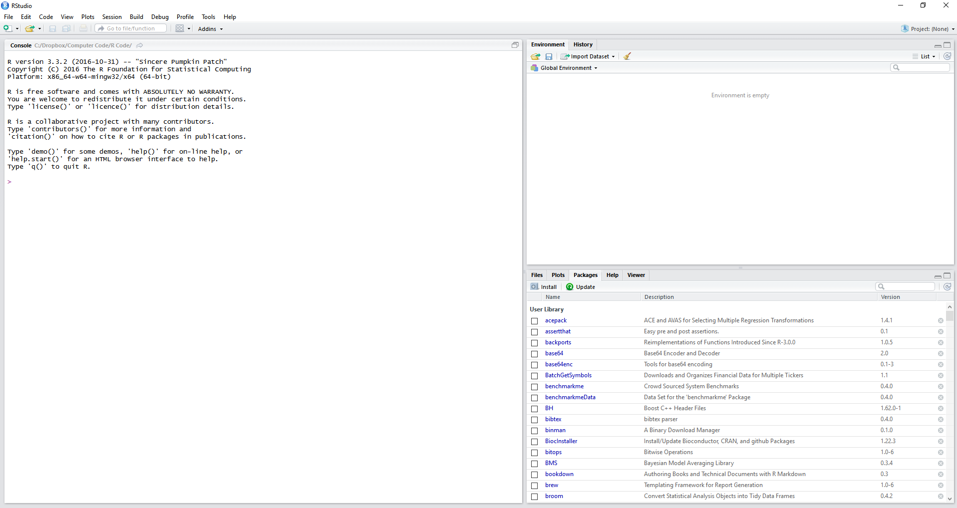
Figure 2.1: The RStudio screen
Note that RStudio automatically detected the installation of R and initialized a session on the left side of the interface.
As a first exercise, click File, New File, and R Script. A text editor should appear on the left side of the screen. It is there that we will spend most of our time developing code. Commands are executed sequentially, from top to bottom. A side note, all .R files created in RStudio are just text files and can be edited anywhere. As an exercise, use Windows’s Notepad to open an R file. You’ll see that the raw code is the same, but without the syntax highlighting.
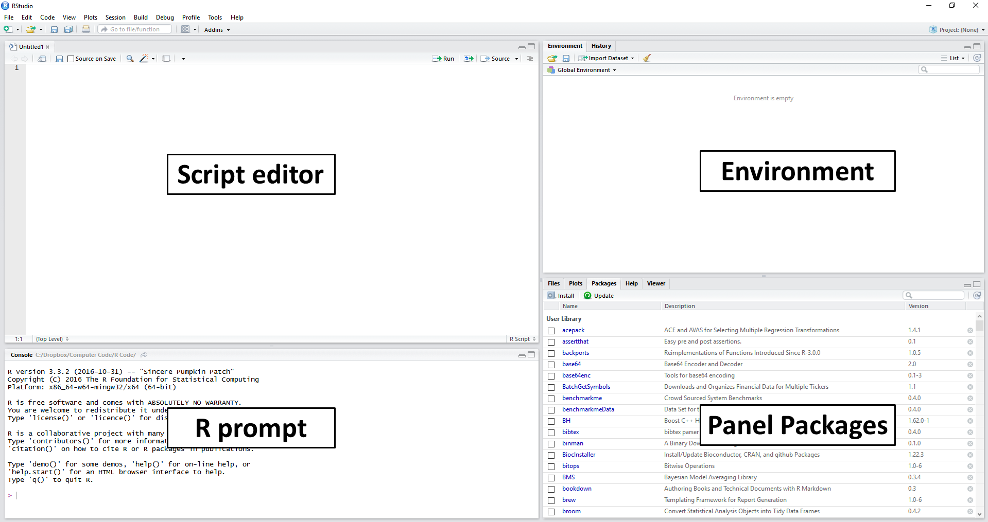
Figure 2.2: Explaining the RStudio screen
When using RStudio, a common suggestion is to change the color scheme to a dark mode setting. It is not just an aesthetic issue, but also a strategy for preventing eye strain. Since you will be spending a lot of time in front of the computer, it is smart to change the colors of the interface to relieve your eyes of the constant brightness of the screen. That way, you’ll be able to work longer, without straining your vision. You can configure the color scheme of RStudio by going to the option Tools, Global Options and then Appearance. A dark color scheme that I personally like and suggest is Ambience.
After the previous steps in RStudio, the resulting screen should look like the image in Figure 2.2. The main items/panels are:
Script Editor: located on the left side and above the screen. This panel is used to write scripts and functions, mostly on files with the .R extension;
R prompt: on the left side and below the script editor. It displays the prompt, which can also be used to give commands to R. The main purpose of the prompt is to test code and display the results of the commands entered in the script editor;
Environment: located on the top-right of the screen. Shows all objects, including variables and functions, currently available to the user. Also note a History panel, which shows the history of commands previously executed by the user;
Panel Packages: shows the packages installed and loaded by R. Here you have four tabs: Files, to load and view system files; Plots, to view statistical figures created in R; Help to access the help system and Viewer to display dynamic and interactive results, such as a web page.
As an introductory exercise, let’s initialize two objects in R. Inside the prompt (lower left side), insert these commands and press enter at the end of each. The <- symbol is nothing more than the result of joining < (less than) with the - (minus sign). The ' symbol represents a single quotation mark and, in most computer keyboards, it is found under the escape (esc) key (top left).
# set x
x <- 1

# set y
y <- 'My humble text'
If done correctly, notice that two objects are available in the environment panel, one called x with a value of 1, and another called y with the text content "My humble text". Also noticed how we used specific symbols to define objects x and y. The use of double quotes (" ") or single quotes (' ') defines objects of the class character. Numbers are defined by the value itself. As will be discussed later, understanding R object classes are important as each has a different behavior within the R code. After executing the previous commands, notice that the history tab has been updated.
Now, lets show the values of x on the screen. To do this, type the following command:
# print contents of x
print(x)
R> [1] 1The print() function is one of the main commands for displaying values in the prompt of R. The text displayed as [1] indicates the index of the first line number. To verify this, enter the following command, which will show a lengthy sequence of numbers on the screen:
# print a sequence
print(50:100)
R> [1] 50 51 52 53 54 55 56 57 58 59 60 61 62 63
R> [15] 64 65 66 67 68 69 70 71 72 73 74 75 76 77
R> [29] 78 79 80 81 82 83 84 85 86 87 88 89 90 91
R> [43] 92 93 94 95 96 97 98 99 100Here, we use the colon symbol in 50:100 to create a sequence starting at 50 and ending at 100. Note that, on the left side of each line, we have the values [1], [13], and [25]. These represent the index of the first element presented in the line. For example, the fifteenth element of 50:100 is 64.
2.6 R Packages
One of the greatest benefits of using R is its package collection. A package is nothing more than a group of procedures aimed at solving a particular computational problem. R has at its core a collaborative philosophy. Users provide their codes for others to use. And, most importantly, all packages are free. For example, consider the scenario where a user is interested in accessing data about historical inflation in the USA. He can install and use an R module that is specifically designed for importing data from central banks and research agencies.
Every function in R belongs to a package. When R initializes, packages stats, graphics, grDevices, utils, datasets, methods and base are loaded by default. This is way why we can use some functions in R without the explicit call to a library. For example, function print is from the base package and is available whenever you start R.
R packages can be accessed and installed from different sources. The main being CRAN (The Comprehensive R Archive network), and Github. It’s worth knowing that the quantity and diversity of R packages increases every day. CRAN is the official repository of R and it is built and maintained by the community. One of the reasons for the success of CRAN is the quality of code. While anyone can send a package, there is an evaluation process to ensure that certain strict rules about code format and safety are respected. For those interested in creating and distributing packages in CRAN, a clear roadmap on is available on the R packages site27. The official (and complete) rules are available on the CRAN website28.
So far, I have eight package published in CRAN. In my experience, sending and publishing a package on CRAN can demand a significant amount of work, especially in the first submission. After that, it becomes a lot easier. Don’t be angry if your package is rejected. My own packages were rejected several times before entering CRAN. Listen to what the maintainers tell you and try fixing all problems before resubmitting. If you’re having issues that you cannot solve or find a solution on the Internet, look for help in the R-packages mailing list1. You’ll probably be surprised at how accessible and helpful the R community can be.
The complete list of packages available on CRAN, along with a brief description of each, can be accessed at the packages section of the R site29. A practical way to check if there is a package that does a specific procedure is to load the previous page and search in your browser for a keyword of interest (e.g. “SEC data”). If there is a package that does what you want, it is very likely that the keyword is used in the description field.
Another important source for finding packages is the CRAN Task Views30. There you can find the collection of noteworthy packages for a given area of expertise. See the Task Views screen in Figure 2.3.
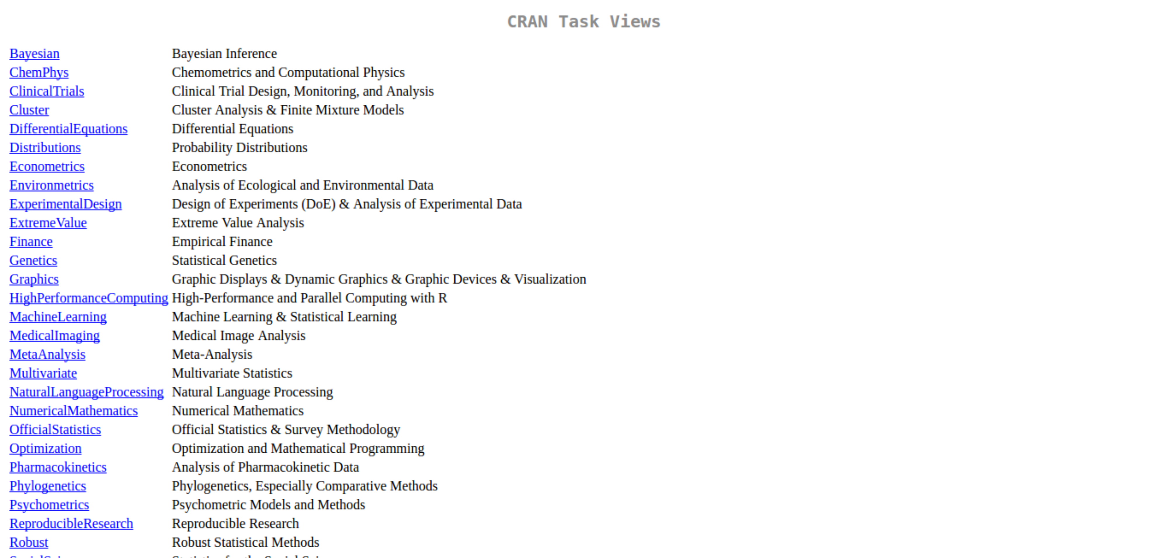
Figure 2.3: Task View screen
A popular alternative to CRAN is Github31. Unlike the former, Github imposes no restrictions on the submitted code and, because of this flexibility and its version control system, it is a popular choice by developers. In practice, it is very common for developers to maintain a development version of a module on Github and the official version in CRAN. When the development version reaches a certain stage of maturity, it is then sent to CRAN.
The most interesting part about R packages is that they can be installed directly from the prompt using the internet. To find out the current amount of packages on CRAN, type and execute the following commands in the prompt:
# get a matrix with available packages
df_cran_pkgs <- available.packages()

# find the number of packages
n_cran_packages <- nrow(df_cran_pkgs)

# print it
print(n_cran_packages)
R> [1] 20186Currently, 2023-12-13 10:30:15.688163, there are 20186 packages available on the CRAN servers, a very impressive mark for the community of developers as a whole.
You can also check the amount of locally installed packages in R with the installed.packages() command:
# find number of packages currently installed
n_local_packages <- nrow(installed.packages())

# print it
print(n_local_packages)
R> [1] 546In this case, the computer in which the book was compiled has 546 packages currently installed. Notice that, even as an experienced R programmer, I’m only using a small fraction of all packages available in CRAN!
2.6.1 Installing Packages from CRAN
Use command install.packages() to install a package locally. You only need to do it once for each new package. As an example, we will install a package called {readr} (Wickham, Hester, and Bryan 2023), that will be used in future chapters. Note that we defined the package name in the installation as if it were text with the use of quotation marks (" ").
# install package readr
install.packages("readr")
That’s it! After executing this simple command, package {readr} (Wickham, Hester, and Bryan 2023) will be installed and the functions related to the package will be ready for use once the package is loaded in a script. If the installed package is dependent on another package, R detects this dependency and automatically installs the missing packages. Thus, all the requirements for using the installed package are satisfied and everything will work perfectly. Be aware, however, that some modules can require external software in the level of the operating system. These cases are usually announced in the description of the package and an error informs that a requirement is missing. External dependencies for R packages are not common, but they do happen.
2.6.2 Installing Packages from Github
To install a package hosted in Github, you must first install the {devtools} (Wickham et al. 2022) package, available on CRAN:
# install devtools
install.packages('devtools')
After that, use function devtools::install_github() to install a package directly from Github. In the following example, we will install the development version of package {dplyr} (Wickham, François, et al. 2023):
# install ggplot2 from github
devtools::install_github("hadley/dplyr")
Note that the username of the developer is included in the input string. In this case, the hadley name belongs to the developer of {dplyr} (Wickham, François, et al. 2023), Hadley Wickham. Throughout the book, you will notice that this name appears several times. Hadley is a prolific and competent developer of several popular R packages and currently works for RStudio.
Be aware that github packages are not moderated. Anyone can send code there and the content is not independently checked. Never install github packages without some confidence of the author’s work. Although unlikely - it never happened to me, for example - it is possible that they have malicious code.
2.6.3 Loading Packages
Within a script, use function library() to load a package, as in the following example.
After running this command, all functions of the package will be available in the current R session. Whenever you close RStudio or start a new session, you’ll lose all loaded packages. This is the reason why packages are usually loaded in the top of the script: starting from a clean memory, required packages are sequentially loaded before the actual R code is executed.
If the package you want to use is not available, R will throw an error message. See an example next, where we try to load a non-existing package called unicorn.
library(unicorn)R> Error in library(unicorn): There is no package called "unicorn"Remember this error message. It will appear every time a package is not found. If you got the same message when running code from this book, you need to check what are the required packages of the example and install them using install.packages() .
Alternatively, if you want to use a specific function and do not want to load all functions from the same package, you can do it with the use of double colons (::), as in the following example.
# example of using a function without loading package
fortunes::fortune(10)
R>
R> Overall, SAS is about 11 years behind R and S-Plus in
R> statistical capabilities (last year it was about 10 years
R> behind) in my estimation.
R> -- Frank Harrell (SAS User, 1969-1991)
R> R-help (September 2003)Here, we use function fortunes::fortune() from the package {fortunes} (R-fortunes?), which shows on screen a potentially funny phrase chosen from the R mailing list. For our example, we selected message number 10. One interesting use of package {fortunes} (R-fortunes?) is to display a random joke every time R starts and, perhaps, lighten up your day. As mentioned before, R is fully customizable. You can find many tutorials on how to achieve this effect by searching on the web for “customizing R startup”.
Another way of loading a package is by using the require() function. A call to require() has a different behavior than a call to library() . Whenever you try to load an uninstalled package with the library() function, it returns an error. This means that the script stops and no further code are evaluated. As for require() , if a package is not found, it returns an object with value FALSE and the rest of the code is evaluated. So, in order to avoid code being executed without its explicit dependencies, it is best advised to always use library() for loading packages in R scripts.
The use of require() is left for loading up packages inside of functions. If you create a custom function that requires procedures from a particular package, you must load the package within the scope of the function. For example, see the following code, where we create a new function called fct_example that depends on the package {quantmod} (Ryan and Ulrich 2023):
fct_example <- function(x){

  require(quantmod)

    df <- getSymbols(x, auto.assign = F)
    return(df)
}
In this case, the first time that fct_example is called, it loads up the package {quantmod} (Ryan and Ulrich 2023) and all of its functions. Using require() inside a function is a good programming policy because the function becomes self-contained, making it easier to use it in the future. This was the first time where the complete definition of a user-created function in R is presented. Do not worry about it for now. We will explain it further in chapter 8.
Be aware that loading a package can cause a conflict of
functions. For example, there is a function called
filter in the dplyr package and also in the
stats package. If we load both packages and call the
filter function within the scope of the code, which one
will R use?
Well, the preference is always for the last loaded
package. This is a type of problem that can be very confusing.
Fortunately, note that R itself tests for conflicts when loading a
package. Try it out: start a new R session and load the
dplyr package. You’ll see that a message indicates that
there are two conflicts with the stats package – functions
filter and lag – and four with the
base package.
A simple strategy to avoid bugs due to conflict of function is to
call a function using the actual package name. For example, if I’m
calling lag from dplyr, I can write the call
as dplyr::lag. As you can see, the package name is
explicit, avoiding any possible conflict.
2.6.4 Upgrading Packages
Over time, it is natural that packages available on CRAN are upgraded to accommodate new features and fix bugs. Thus, it is recommended that users update their installed packages to a new version. In R, a simple and direct way of upgrading packages is to click the button Update located in the package panel, lower right corner of RStudio, as shown in Figure 2.4.
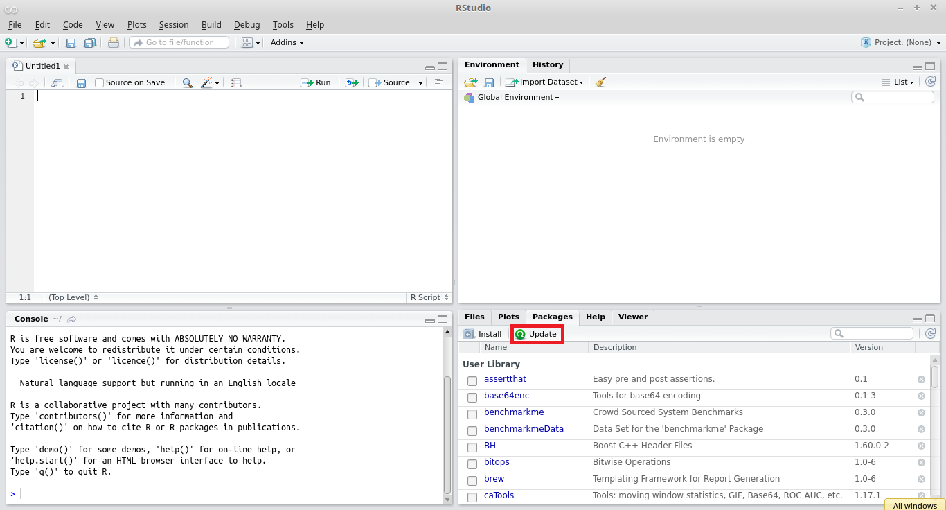
Figure 2.4: Updating R packages
The user can also update packages using commands. Simply type command update.packages() and hit enter, as shown below.
# update all installed packages
update.packages()
The command update.packages() compares the version of the installed packages with the versions available in CRAN. If it finds any difference, the new version is downloaded and installed. After running the command, all packages will be synchronized with the versions available in CRAN.
Package versioning is an extremely important topic for keeping your code reproducible. Although it is uncommon to happen, a new package version can change the results of your analysis. I have a particularly unpleasant experience when a scientific article returned from a journal review and, due to the update of one of the R packages I used, I was unable to reproduce the results presented in the article. In the end everything went well, but the trauma remains.
One solution to this problem is to freeze the package versions for
each project using RStudio’s renv tool. In summary,
renv makes local copies of the packages used in the
project, which have preference over system packages. Thus, if a package
is updated in the system, but not in the project, the R code will
continue to use the older version and the R code will always run under
the same conditions.
2.7 Running Scripts from RStudio
Now, let’s copy some code into the editor’s screen (upper left side). The result should look like Figure 2.5.
# a complete script
x <- 1
y <- "my humble text"
print(x)
R> [1] 1
print(y)R> [1] "my humble text"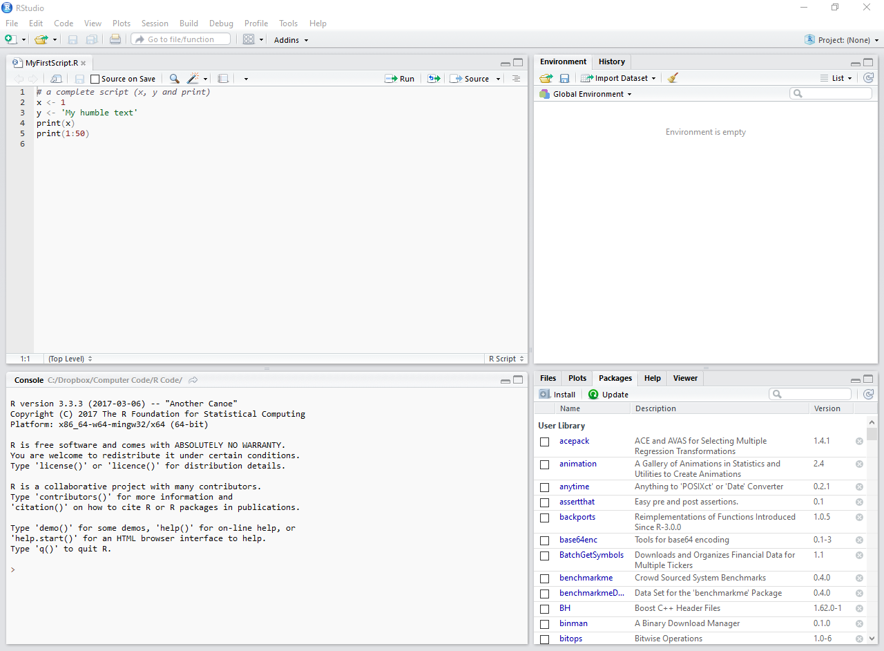
Figure 2.5: Example of an R script
After pasting all the commands in the editor, save the .R file to a personal folder where you have read and write permissions. In Windows, one possibility is to save it in the Documents folder with a name like 'my_first_script.R'. This saved file, which at the moment does nothing special, records the steps of a simple algorithm that creates several objects and shows their content.
2.8 Using the help files
There is no shame in seeking help. Advanced R users often seek instructions on specific tasks, whether it is to better understand the execution details of some functions or simply to study a new procedure. The use of the R help system is part of the work and you should master it as soon as possible.
Within RStudio, you can get help by using the help panel in RStudio or directly from the prompt. Simply enter the question mark next to the object on which you want help, as in ?mean. In this case, object means is a function and the use of the help() command will open a panel on the right side of RStudio. Another way of opening the help page of a function is the select the name of the function and press F1 in the keyboard.
In R, the help screen of a function is the same as shown in Figure 2.6. It presents a general description of the function, explains its input arguments and the format of the output. The help screen follows with references and suggestions for other related functions. More importantly, examples of usage are given last and can be copied to the prompt or script in order to accelerate the learning process.
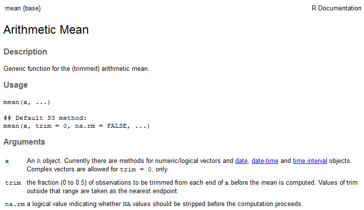
Figure 2.6: Help screen for function mean
If we are looking for help for a given text and not a function name, we can use double question marks as in ??"standard deviation". This operation will search for the occurrence of the term in all packages of R and it is very useful to learn how to perform a particular task. In this case, we looked for the available functions to calculate the standard deviation of a vector.
As a suggestion, the easiest and most direct way to learn a new function is by trying out the examples in the manual. This way, you can see which types of inputs the function expects and what type of output it provides back. Once you have it working in your code, read the help screen to understand if it does exactly what you expected and what are the options for its use. If the function performs the desired procedure, you can copy and paste the example for your own script, adjusting where necessary.
Another very important source of help is the Internet itself. Sites like stackoverflow32 and specific mailing lists and blogs, whose content is also on the Internet, are a valuable source of information. If you find a problem that could not be solved by reading the standard help files, the next logical step is to seek a solution using your error message or the description of the problem in search engines. In many cases, your problem, no matter how specific it is, has already occurred and has been solved by other users. In fact, it is more surprising not to find the solution for a programming problem on the internet, than the other way around.
Whenever you ask for help on the internet, always try to 1) describe your problem clearly and 2) add a reproducible code of your problem. Thus, the reader can easily verify what is happening by running the example on his computer, and solving the problem.
2.8.1 RStudio shortcuts
In RStudio, there are some predefined and time-saving shortcuts for running code from the editor. To execute an entire script, simply press control + shift + s. This is the source command. With RStudio open, I suggest testing this key combination and checking how the code saved in a .R file is executed. The output of the script is shown in the prompt of R. The result in RStudio should look like Figure 2.7.
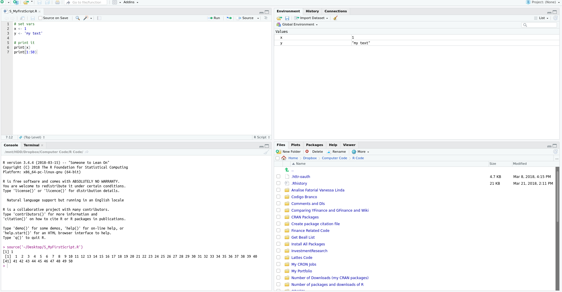
Figure 2.7: Example of a R script after execution
Another way of executing code is with the shortcut control + enter, which will only execute the line where the cursor is located. This shortcut is very useful in developing scripts because it allows each line of the code to be tested. As an example of usage, point the cursor to the print(x) line and press control + enter. As you will notice, only the line print(x) was executed and the cursor moves to the next line. Therefore, before running the whole script, you can test it line by line and check for possible errors.
Next, I highlight these and other RStudio shortcuts, which are also very useful.
- control + shift + s
- executes (source) the current RStudio file;
- control + shift + enter
- executes the current file with echo, showing the commands on the prompt;
- control + enter
- executes the selected line, showing on-screen commands;
- control + shift + b
- executes the codes from the beginning of the file to the cursor’s location;
- control + shift + e
- executes the codes of the lines where the cursor is until the end of the file.
I suggest you try to create a healthy habit by using these shortcuts from day one. Those who like to use the mouse, an alternate way to execute code is to click the source button in the upper-right corner of the code editor.
If you want to run code in a .R file within another .R file, you can use the source() command. For example, imagine that you have a main R script with your data analysis and another two scripts that performs some support operation such as importing data to R. These operations have been dismembered as a way of organizing the code.
To run the support scripts, just call it with function source in the main script, as in the following code:
Here, all code in 01-import-data.R and 02-build-tables.R will be executed sequentially. This equals manually opening each file and hitting control + shift + s.
2.9 Testing and Debugging Code
Developing code follows an observable cycle. At first, you will write a command line on a script, try it using control + enter, and check the result on the prompt or the content of objects. A new line of code is written once the previous line worked as expected. A moving cycle is clear, writing code is followed by line execution, followed by result checking, modify and repeat if necessary. This is a normal and expected process. You need to make sure that every line of code is correctly specified before moving to the next one. Whenever the code asks for something that is not expected (or possible), an error occurs.
When trying to find an error in a preexisting script, R offers debugging tools for controlling and assessing its execution. This is especially useful when you have a long and complicated script. The simplest and easiest tool that R and RStudio offer is code breakpoint. In RStudio, you can click on the left side of the script editor and a red circle will appear, as in Figure 2.8.
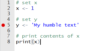
Figure 2.8: Example of breakpoint in an R script
This red circle indicates a flag that will force the code to stop at that line. You can use it to test existing code and check its objects at a certain part of the execution. Pausing the code at a certain point might seem strange for a starting programmer but, for large scripts, with many functions and complex code, it is a necessity. When the execution hits the breakpoint, the prompt will change to Browse[1]> and you’ll be able to try new code and verify the content of all current objects. From the Console, you have the option to continue the execution to the next breakpoint or stop it by pressing shift+f8. The same result can be achieved using a function called browser. Have a look:
The practical result is the same as using RStudio’s red circle, but it gives you more control for the case of several commands in the same line.
2.10 Creating Simple Objects
One of the most basic and most used commands in R is the creation of objects. As shown in previous sections, you can define an object using the <- command, which is verbally translated to assign. For example, consider the following code:
# set x
x <- 123

# set my_x, my_y and my_z in one line
my_x <- 1; my_y <- 2; my_z <- 3
We can read this code as the value 123 is assigned to x. The direction of the arrow defines where the value is stored. For example, using 123 -> x also works, although this is not recommended as the code becomes less readable. Moreover, notice that you can create objects within the same line by separating the commands using a semi-colon.
Using an arrow symbol <- for object definition is a
simple way to identify R code. The reason for this choice was that, at
the time of conception of the S language, keyboards had a
specific key that directly defined the arrow symbol. This means that the
programmer only had to hit one key in the keyboard to create new
variables. Modern keyboards, however, are different. If you find it
troublesome to type this symbol, you can use a shortcut as well. In
Windows, the shortcut for the symbol <- is
alt plus “-”.
Most programming languages uses a equality symbol (=) to define objects and, often, this creates confusion. When using R, you can also define objects with =, as in x = 123, however, no one should ever recommend it. The equality symbol has a special use within an R code as it defines function arguments, as in my_l <- fct(arg1 = 1, arg2 = 3). For now, just remember to use <- for defining objects. We will learn more about functions and using the equality symbol in a future chapter.
The name of the object is important in R. With the exception of very specific cases, you can name objects as you please. This freedom, however, can work against you. It is desirable to set short object names that make sense to the content of the script and which are simple to understand. This facilitates the understanding of the code by other users and is part of the suggested set of rules for structuring code. Note that all objects created in this book have nomenclature in English and specific format, where the white space between nouns are replaced by an underscore, as in my_x <- 1 and name_of_file <- 'my_data_file.csv'. We will get back at code structure in chapter 13.
R executes code by looking for objects available in the environment, including functions. You also need to be aware that R is case sensitive. That is, object m is not the same as M. If we try to access an object that does not exist, R will return an error message and halt the execution of the rest of the code. Have a look:
print(z)R> Error in eval(expr, envir, enclos): object 'z' not foundThe error occurred because the object z does not exist in the current environment. If we create a variable z as z <- 321 and repeat the command print(z), we will not have the same error message.
2.11 Creating Vectors
In the previous examples, we created simple objects such as x <- 1 and x <- 'ABC'. While this is sufficient to demonstrate the basic commands in R, in practice, such commands are very limited. A real problem of data analysis will certainly have a larger volume of information.
When we gather many elements of the same class, such as numeric, into a single object, the result is an atomic vector. An example would be the representation of a series of daily stock prices as an atomic vector of the class numeric. Once you have a vector, you can manipulate it any way you want.
Atomic vectors are created in R using the c() command, which comes from the verb combine. For example, if we want to combine the values 1, 2 and 3 in a single object, we can do it with the following command:
R> [1] 1 2 3The c() command works the same way for any other class of object, such as character:
R> [1] "text 1" "text 2" "text 3" "text 4"The only restriction when creating vectors is that all elements must have the same class. If we insert data from different classes in a call to c() , R will try to mutate all elements into the same class following its own logic. If the conversion of all elements to a single class is not possible, an error message is returned. Note the following example, where numeric values are set in the first and second element of x and a character in the last element.
R> [1] "1" "2" "3"Notice that all values in x are converted to type character. The use of class() command confirms this result:
# print class of x
class(x)
R> [1] "character"2.12 Knowing Your Environment and Objects
After using various commands, further development of an R script requires you to understand what objects are available and if their content are correct. You can find this information simply by looking at the environment tab in the upper right corner of RStudio. However, there is a command that shows the same information in the prompt. In order to know what objects are currently available in R’s memory, you can use the command ls() . Note the following example:
R> [1] "x" "y" "z"Objects x, y and z were created and are available in the current working environment. If we had other objects, they would also appear in the output to ls() .
To display the content of each object, just enter the names of objects and press enter in the prompt:
# print objects by their name
x
R> [1] 1
yR> [1] 2
zR> [1] 3Typing the object name on the screen has the same effect as using the print() command. In fact, when executing the sole name of a variable in the prompt or script, R internally passes the object to the print() function.
In R, all objects belong to a class. As previously mentioned, to find the class of an object, simply use the class() function. In the following example, x is an object of the class numeric, y is a text (character) object and fct_example is a function object.
R> [1] "numeric"R> [1] "character"R> [1] "function"Another way to learn more about an object is to check its textual representation. Every object in R has this property and we can find it with function str() :
R>  int [1:10] 1 2 3 4 5 6 7 8 9 10
R> NULL
We find that object x is a vector of class int (integer). Function str() is particularly useful when trying to understand the details of a more complex object, such as a dataframe or a list, which will be introduced in future chapter.
2.13 Finding the Size of Objects
In R, an object size can mean different things but most likely it is defined as the number of individual elements that constitute the object. This information serves not only to assist the programmer in checking possible code errors but also to know the length of iteration procedures such as loops, which will be treated in a later chapter of this book.
In R, the size of an object can be checked with the use of four main functions: length() , nrow() , ncol() and dim() .
Function length() is intended for objects with a single dimension, such as atomic vectors:
# create atomic vector
x <- c(2, 3, 3, 4, 2,1)

# get length of x
n <- length(x)

# display message
message('The length of x is ', n)
R> The length of x is 6For objects with more than one dimension, such as a matrix, use functions nrow() , ncol() and dim() (dimension) to find the number of rows (first dimension) and the number of columns (second dimension). See the difference in usage below.
R>      [,1] [,2] [,3] [,4] [,5]
R> [1,]    1    5    9   13   17
R> [2,]    2    6   10   14   18
R> [3,]    3    7   11   15   19
R> [4,]    4    8   12   16   20
# calculate size in different ways
my_nrow <- nrow(M)
my_ncol <- ncol(M)
my_n_elements <- length(M)

# display messages
message('The number of lines in M is ', my_nrow)
R> The number of lines in M is 4
message('The number of columns in M is ', my_ncol)R> The number of columns in M is 5
message('The number of elements in M is ', my_n_elements)R> The number of elements in M is 20The dim() function shows the dimension of the object, resulting in a numeric vector as output. This function should be used when the object has more than two dimensions. In practice, however, such cases are rare as most data-related problems can be solved with a bi-dimensional representation. An example is given next:
R> [1] 4 5In the case of objects with more than two dimensions, we can use the array() function to create the object and dim() to find its size. Have a look at the next example:
# create an array with three dimensions
my_array <- array(1:9, dim = c(3, 3, 3))

# print it
print(my_array)
R> , , 1
R>
R> [,1] [,2] [,3]
R> [1,] 1 4 7
R> [2,] 2 5 8
R> [3,] 3 6 9
R>
R> , , 2
R>
R> [,1] [,2] [,3]
R> [1,] 1 4 7
R> [2,] 2 5 8
R> [3,] 3 6 9
R>
R> , , 3
R>
R> [,1] [,2] [,3]
R> [1,] 1 4 7
R> [2,] 2 5 8
R> [3,] 3 6 9R> [1] 3 3 32.14 Selecting Elements from an Atomic Vector
After creating an atomic vector, you can access and select portions of it. For example, suppose that a month ago you invested 1.000 USD in Apple shares. You download stock price data for previous month and want to see how much your portfolio is currently worth. In that case, you are interested only in latest price of the stocks. All price values from other dates are not relevant to our analysis and therefore could be safely ignored.
The selection of pieces of an atomic vector is called indexing and it is accomplished with the use of square brackets ([ ]). Consider the following example:
# set x
my_x <- c(1, 5, 4, 3, 2, 7, 3.5, 4.3)
If we wanted only the third element of my_x, we use the bracket operator as follows:
# get the third element of x
elem_x <- my_x[3]

# print it
print(elem_x)
R> [1] 4Indexing also works using vectors containing the desired locations. If we are only interested in the last and penultimate values of my_x, we use the following code:
# set vector with indices
my_idx <-  (length(my_x)-1):length(my_x)

# get last and penultimate value of my_x
piece_x_1 <- my_x[my_idx]

# print it
print(piece_x_1)
R> [1] 3.5 4.3A cautionary note: a unique property of the R language is that if a non-existing element of an object is accessed, the program returns the value NA (not available). See the next example code, where we attempt to obtain the fourth value of a vector with only three components.
R> [1] NAThis is important because NA elements are contagious. That is, anything that interacts with NA will also become NA. The lack of treatment of these errors can lead to problems that are difficult to identify. In other programming languages, attempting to access non-existing elements generally returns an error and cancels the execution of the rest of the code.
In most cases, the occurrence of NA (Not
Available) values suggests that a problem exists within the code.
Always remember that NA values indicates lack of data and
are contagious: anything that interacts with a NA value
will turn into another NA. You should become
suspicious about your code quality every time that NA
values are found unexpectedly.
The use of indices is very useful when you are looking for items of a vector that satisfy some condition. For example, if we wanted to find out all values in my_x that are greater than 3, we could use the following command:
# find all values in my_x that is greater than 3
piece_x_2 <- my_x[my_x>3]

# print it
print(piece_x_2)
R> [1] 5.0 4.0 7.0 3.5 4.3It is also possible to index elements by more than one condition using the logical operators & and | (or). For example, if we wanted the values of my_x greater than 2 and lower than 4, we could use the following command:
# find all values of my_x that are greater than 2 and lower then 4
piece_x_3 <- my_x[ (my_x > 2) & (my_x < 4) ]
print(piece_x_3)
R> [1] 3.0 3.5Likewise, if we wanted all items that are lower than 3 or greater than 6, we use:
# find all values of my_x that are lower than 3 or higher than 6
piece_x_4 <- my_x[ (my_x < 3) | (my_x > 6) ]

# print it
print(piece_x_4)
R> [1] 1 2 7Moreover, logic indexing also works with the interaction of different objects. That is, we can use a logical condition in one object to select items from another:
# set my_x and my.y
my_x <- c(1, 4, 6, 8, 12)
my_y <- c(-2, -3, 4, 10, 14)

# find all elements of my_x where my.y is higher than 0
my_piece_x <- my_x[my_y > 0 ]

# print it
print(my_piece_x)
R> [1] 6 8 12Looking more closely at the indexing process, notice that we are creating a variable of the logical type. This object takes only two values: TRUE and FALSE. Have a look in the code presented next, where we create a logical object, print it and present its class.
# create a logical object
my_logical <- my_y > 0

# print it
print(my_logical)
R> [1] FALSE FALSE TRUE TRUE TRUE
# find its class
class(my_logical)
R> [1] "logical"Logical objects are very useful whenever we are testing a particular condition on a data set. We will learn more about this and other basic classes in chapter 7.
2.15 Removing Objects from the Memory
After creating several variables, the R environment can become full of used and disposable content. In this case, it is desirable to clear the memory to erase objects that are no longer needed. Generally, this is accomplished at the beginning of a script, so that every time the script runs, the memory will be cleared before any calculation. In addition to cleaning the computer’s memory, it also helps to avoid possible errors in the code.
For example, given an object x, we can delete it from memory with the command rm() , as shown next:
# set x
x <- 1

# remove x
rm('x')
After executing the command rm('x'), the value of x is no longer available in the R session. In practical situations, however, it is desirable to clean up all the memory used by all objects created in R. We can achieve this goal with the following code:
The term list in rm(list = ls()) is a function argument of rm() that defines which objects will be deleted. The ls() command shows all the currently available objects. Therefore, by chaining together both commands, we erase all current objects available in the environment. As mentioned before, it is a good programming policy to clear the memory before running the script. However, you should only wipe out all of R’s memory if you have already saved the results of interest or if you can replicate them.
Clearing memory in scripts is a controversial topic. Some authors argue that it is better not to clear the memory as this can erase important results. My opinion is that it is important to clear the memory at the top of the script, as long as all results are reproducible. When you start a code in a clean state – no variables or functions – it becomes easier to understand and solve possible bugs.
2.16 Displaying and Setting the Working Directory
Like other programming platforms, R always executes code in a working directory. If no directory is set, a default value is used when R starts up. It is based on the working directory that R searches for files to load data or other R scripts. It is in this directory that R saves any output if we do not explicitly define a path on the computer. This output can be a graphic file, text or a spreadsheet. That said ,it is good policy to change the working directory to the same place where the script is located.
The simplest way of checking the current working directory is looking at RStudio’s prompt panel. At the top, in a small font and just below the word “Console”, you’ll see the working path. Using code, we can check the current working directory with function getwd() :
R> C:/my-books/afedR-ed4/book-contentThe result of the previous code shows the folder in which this book was written and compiled.
The change of the working directory is performed with the setwd() command. For example, if we wanted to change our working directory to C:/My Research/, simply type in the prompt:
# set where to change directory
my_d <- 'C:/My Research/'

# change it
setwd(my_d)
After changing the directory, importing and saving files in the C:/My Research/ folder will be a lot easier.
Additionally, the easiest and most straightforward way to ensure that the working directory is the same as the R script is using RStudio projects. To do so, click in “File” and “New Project”. Doing so will create a .Rproj file in the chosen directory of the project. The trick here is to create the R scripts in the root folder of the project. Every time you open the project, it will automatically change the working directory to where the .Rproj file is located.
Once you are working on the same path as the script, using relative paths is preferable. For example, if you are working in a folder that contains a subdirectory called data, you can enter this sub-folder with the code:
# change to subfolder
setwd('data')
Another possibility is to go to a previous level of the directory using .., as in:
# change to the previous level
setwd('..')
So, if you are working in directory C:/My Research/ and execute the command setwd('..'), the current folder becomes C:/, which is one level below C:/My Research/.
2.17 Canceling Code Execution
Whenever R is running some code, a visual cue in the shape of a small red circle with the word stop in the right corner of the prompt will appear. This button is not only an indicator that R is busy running code but also a shortcut for canceling its execution. Another way to cancel an execution is to point the mouse to the prompt and press the escape (esc) button from the keyboard.
To try it out, run the next chunk of code in RStudio and cancel its execution using esc.
In the previous code, we used a for loop and function Sys.sleep to display the message '\nRunning code (please make it stop by hitting ESC!)' one hundred times, every second. For now, do not worry about the code and functions used in the example. We will discuss the use of loops in chapter 8.
Another very useful trick for defining working directories in R is to
use the ~ symbol. The tilda defines the “Documents” folder
in Windows, which is unique for each user. For Linux and Mac
users, the tilda defines the “home” folder (e.g. “/home/USERNAME”).
Therefore, by running setwd(‘~’), you will direct R to a
personal folder in any operating system.
2.18 Code Comments
In R, comments are set using the hashtag symbol #. Any text after this symbol will not be processed. This gives you the freedom to write whatever you want within the script. An example:
# this is a comment (R will not parse it)
# this is another comment (R will again not parse it)

x <- 'abc' # this is an inline comment
Comments are an effective way to communicate any important information that cannot be directly inferred from the code. In general, you should avoid using comments that are too obvious or too generic:
# read CSV file
df <- read.csv('data/data_file.csv')
As you can see, it is quite obvious from the line df <- read.csv('..') that the code is reading a .csv file. The name of the function already states that. So, the comment was not a good one as it did not add any new information to the user. A better approach at commenting would be to set the author, description of the script and better explain the origin and last update of the data file. Have a look:
# Script for reproducing the results of JOHN (2019)
# Author: Mr data analyst (dontspamme@emailprovider.com)
# Last script update: 2020-01-10
#
# File downloaded from www.site.com/data-files/data_file.csv
# The description of the data goes here
# Last file update: 2020-01-10

df <- read.csv('data/data_file.csv')
So, by reading the comments, the user will know the purpose of the script, who wrote it and the date of the last edit. It also includes the origin of the data file and the date of the latest update. If the user wants to update the data, all he has to do is go to the referred website and download the new file.
Another productive use of comments is to set sections in the code, such as in:
# Script for reproducing the results of JOHN (2019)
# Author: Mr data analyst (dontspamme@emailprovider.com)
# Last script update: 2020-01-10
#
# File downloaded from www.site.com/data-files/data_file.csv
# The description of the data goes here
# Last file update: 2020-01-10

# Clean data -------------------------
# - remove outliers
# - remove unnecessary columns

# Create descriptive tables ----------


# Estimate models --------------------


# Report results ---------------------
The use of a long line of dashes (-) at each section of the code is intentional. It causes RStudio to identify and bookmark the sections, with a link to them at the bottom of the script editor. Test it yourself, copy and paste the above code into a new R script, save it, and you’ll see that the sections appear on a button between the editor and the prompt. Such a shortcut can save plenty of time in lengthy scripts.
When you start to share code with other people, you’ll soon realize that comments are essential and expected. They help transmit information that is not available from the code. This is one way of a discerning beginners from experienced programmers. Contrary to popular belief, it is likely that someone with experience in programming will be very communicative in its comments (sometimes too much!). A note here, throughout the book you’ll see that the code comments are, most of the time, a bit obvious. This was intentional as clear and direct messages are important for new users, which is part of the audience of this book.
2.19 Using Code Completion with tab
A very useful feature of RStudio is code completion, an editing tool that facilitates the search of object names, packages, function arguments, and files. Its usage is very simple. After you type any first letter in the keyboard, just press tab (left side of the keyboard, above capslock) and a number of options will appear. See Figure 2.9 where, after entering the f letter and pressing tab, a small window appears with a list of object names that begin with that letter.
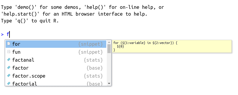
Figure 2.9: Usage of autocomplete for object name
The autocomplete feature is self-aware and will work differently depending on where it is called. As such, it works perfectly for searching for packages. For that, type library() in the prompt or editor, place the cursor in between the parentheses and press tab. The result should look something like Figure 2.10, shown next.
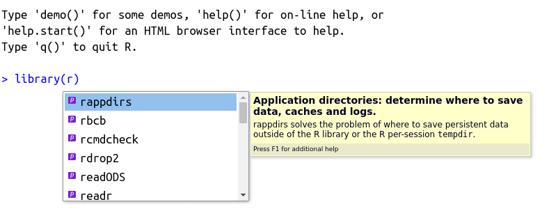
Figure 2.10: Usage of autocomplete for packages
Note that a description of the package or object is also offered by the code completion tool. This greatly facilitates the day to day work as the memorization of package names and R objects can be challenging. The use of the tab decreases the time to look up names, also avoiding possible errors.
The use of this tool becomes even more beneficial when objects and functions are named with some sort of pattern. In the rest of the book, you will notice that objects tend to be named with the prefix my, as my_x, my_num, my_df. Using this naming rule (or any other) facilitates the lookup for the names of objects created by the user. You can just type my_, press tab, and a list of objects will appear.
As mentioned in the previous section, you can also find files and folders on your computer using tab. To try it, write the command my_file <- "" in the prompt or a script, point the cursor to the middle of the quotes and press the tab key. A screen with the files and folders from the current working directory should appear, as shown in Figure 2.11.
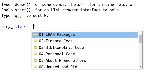
Figure 2.11: Usage of autocomplete for files and folders
The use of autocomplete is also possible for finding the name and description of function arguments. To try it out, write message() and place the mouse cursor inside the parentheses. After that, press tab. The result should be similar to Figure 2.12. By using tab inside of a function, we have the names of all arguments and their description – a mirror of the information found in the help files.
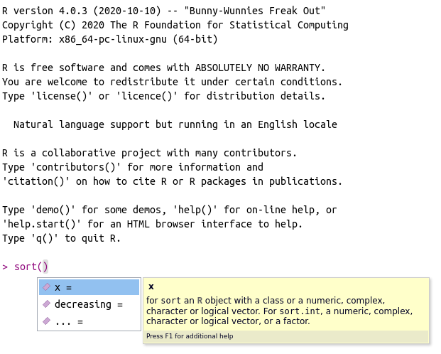
Figure 2.12: Usage of autocomplete for function arguments
Likewise, you can also search for a function within a package with tab. For that, simply type the name of the package followed by two commas, as in readr::, and press tab. The result should be similar to Figure 2.13
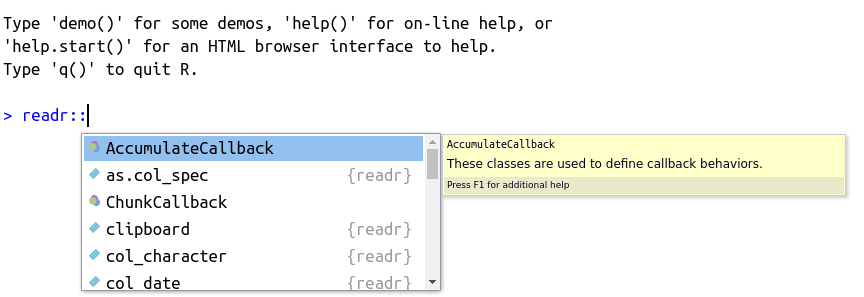
Figure 2.13: Usage of autocomplete for finding functions within a package
Summing up, using code completion will make you more productive. You’ll find names of files, objects, arguments, and packages much faster. Use it as much as you can.
Autocomplete is one of the most important tools of RStudio, helping users to find object names, locations on the hard disk, packages and functions. Get used to using the tab key and, soon enough, you’ll see how much the autocomplete tool can help you write code quickly, and without typos.
2.20 Interacting with Files and the Operating System
As you are learning R, soon enough you’ll find a data-related problem that requires some interaction with files on the computer, either by creating new folders, decompressing and compressing files, listing and removing files from the hard drive of the computer or any other type of operation. R has full support for such type of operations. You can automate any type of computer task within an R script, if so needed.
In this section we will give preference to functions from package {fs} (Hester, Wickham, and Csárdi 2023), which provides several routines for interacting with files and folders. Be aware, however, that the base package also offers similar functions.
2.20.1 Listing Files and Folders
To list files from your computer, use function fs::dir_ls() , where the path argument sets the directory to list the files from. For the compilation of the book, I’ve created a directory called data. This folder contains all the data needed to recreate the book’s examples. You can check the files in the sub-folder data with the following code:
R> data/FileWithLatinChar_ISO-8859-9.txt
R> data/FileWithLatinChar_UTF-8.txt
R> data/Financial Sample.xlsx
R> data/MySQLiteDatabase.SQLITE
R> data/SP500-Stocks-WithRet.rds
R> data/SP500-Stocks_long.csv
R> data/SP500-Stocks_wide.csv
R> data/SP500_long_yearly_2010-01-01_2019-11-04.rds
R> data/SQLite_db.SQLITE
R> data/UCI_Credit_Card.csv
R> data/price-data.csv
R> data/pride_and_prejudice.txt
R> data/temp.txt
R> data/temp_file.xlsx
R> data/top25babynames-by-sex-2005-2017.csv
There are several files with different extensions in this directory. These files contain data that will be used in future chapters.
You can also list the files recursively over inner folders, that is, list all files from all sub-folders contained in the original path. To check it, try using the following code in your computer:
# list all files for all subfolders (IT MAY TAKE SOME TIME...)
fs::dir_ls(path = getwd(), recurse = TRUE)
The previous command will list all files in the current folder and sub-folders. Depending on the current working directory, it may take some time to run it all (you can cancel it anytime by pressing esc in your keyboard).
You can also set what type of output you need. For example, if you want only the available folders, and not files, use input type = "directory":
# store names of directories
my_dirs <- fs::dir_ls(
    path = getwd(),
    type = "directory")

# print it
print(my_dirs)
R> /tmp/RtmpCpmYn0/compile-book-html--4f5618cd6e83/_book
R> /tmp/RtmpCpmYn0/compile-book-html--4f5618cd6e83/blocks
R> /tmp/RtmpCpmYn0/compile-book-html--4f5618cd6e83/data
R> /tmp/RtmpCpmYn0/compile-book-html--4f5618cd6e83/ebook files
R> /tmp/RtmpCpmYn0/compile-book-html--4f5618cd6e83/eqs
R> /tmp/RtmpCpmYn0/compile-book-html--4f5618cd6e83/mem_cache
R> /tmp/RtmpCpmYn0/compile-book-html--4f5618cd6e83/quandl_cache
R> /tmp/RtmpCpmYn0/compile-book-html--4f5618cd6e83/resources
R> /tmp/RtmpCpmYn0/compile-book-html--4f5618cd6e83/tabs
R> /tmp/RtmpCpmYn0/compile-book-html--4f5618cd6e83/text-to-reuseThe output shows the directories used to write the book. It includes the directory with the data (“./data”), resources (“./resources”) among others. In this same directory, you can find the chapters of the book, organized by files and based on the RMarkdown language (.Rmd file extension):
# list all files with the extension .Rmd
fs::dir_ls(glob = "*.Rmd")
R> 00a-About-new-edition.Rmd
R> 00b-Preface.Rmd
R> 01-Introduction.Rmd
R> 02-Basic-operations.Rmd
R> 03-Research-scripts.Rmd
R> 04-Importing-exporting-local.Rmd
R> 05-Importing-internet.Rmd
R> 06-Data-structure-objects--ONLINE.Rmd
R> 07-Basic-objects--ONLINE.Rmd
R> 08-Programming--ONLINE.Rmd
R> 09-Cleaning-data--ONLINE.Rmd
R> 10-Figures--ONLINE.Rmd
R> 11-Models--ONLINE.Rmd
R> 12-Reporting-results--ONLINE.Rmd
R> 13-Optimizing-code--ONLINE.Rmd
R> 14-References.Rmd
R> _Welcome.Rmd
R> afedR_ed03_ONLINE.Rmd
R> index.RmdThe files presented above contain all the contents of this book, including this specific paragraph, located in file 02-Basic-operations.Rmd!
2.20.2 Deleting Files and Directories
You can also use an R session to delete files and directories from your computer. This might come in handy when dealing with disposable data files. Use these commands with responsibility. If not careful, you can easily break the operating system of your computer.
You can delete files with command fs::file_delete() :
# create temporary file
my_file <- 'data/tempfile.csv'
write.csv(x = data.frame(x=1:10),
          file = my_file)

# delete it
fs::file_delete(my_file)
To delete directories and all their elements, we use fs::dir_delete() :
# create temp dir
fs::dir_create('temp')

# create a file inside of temp
my_file <- 'temp/tempfile.csv'
write.csv(x = data.frame(x=1:10),
          file = my_file)

fs::dir_delete('temp')
If needed, we can check if the deletion of a directory was successful with command fs::dir_exists() :
fs::dir_exists('temp')R> temp
R> FALSEAs expected, the directory was not found.
2.20.3 Downloading Files from the Internet
We can also use R to download files from the Internet with function download.file() . See the following example, where we download an Excel spreadsheet from Microsoft’s website:
# set link
link_dl <- 'go.microsoft.com/fwlink/?LinkID=521962'
local_file <- 'data/temp_file.xlsx' # name of local file

download.file(url = link_dl,
              destfile = local_file)
Using download.file() is quite handy when you are working with Internet data that is constantly being updated. In the script, we can download new data in every execution, making sure that our analysis is based on current information.
One trick worth knowing is that you can also download files from cloud services such as Dropbox33 and Google Drive34. So, if you need to send a data file to a large group of people and update it frequently, just pass the file link from the cloud service. This way, any local change in the data file in your computer will be reflected for all users with the file link.
Needless to say, be very careful with commands
fs::file_delete and fs::dir_delete, especially
when using recursion (recurse = TRUE). One simple mistake
and important parts of your hard drive can be erased, breaking your
operating system. Be aware that R permanently deletes
files and folder, without any simple way to restore them.
2.20.4 Using Temporary Files and Directories
Every time a user starts an R session, a new temporary folder is created in your hard drive. This folder is used to store any disposable files and folders generated by R. The location of this directory is available with fs::path_temp() :
R> C:\Users\msperlin\AppData\Local\Temp\RtmpEGt3Q7The name of the temporary directory, in this case 'RtmpEGt3Q7', is unique and randomly defined at the start of every new R session. This means that every R session is linked to an unique temporary folder. If two R sessions are created, as in starting two RStudio sessions, two temporary folders will be available, each with an unique name. When the computer is rebooted, all temporary directories are deleted.
The same dynamic is found for file names. If you want to use a temporary random name for some reason, use fs::file_temp() :
R> C:\Users\msperlin\AppData\Local\Temp\RtmpEGt3Q7\file19917e5fbc7eYou can also set its extension and name:
R> C:\Users\msperlin\AppData\Local\Temp\RtmpEGt3Q7\temp_19913e1dafe5.csvAs a practical case of using temporary files and folders, let’s download the Excel worksheet from Microsoft into a temporary folder and read its content for the first five rows:
# set link
link_dl <- 'go.microsoft.com/fwlink/?LinkID=521962'
local_file <- fs::file_temp(ext = '.xlsx')

download.file(url = link_dl,
              destfile = local_file)

df_msft <- readxl::read_excel(local_file)

print(head(df_msft))
R> # A tibble: 6 × 16
R> Segment Country Product `Discount Band` `Units Sold`
R> <chr> <chr> <chr> <chr> <dbl>
R> 1 Government Canada Carretera None 1618.
R> 2 Government Germany Carretera None 1321
R> 3 Midmarket France Carretera None 2178
R> 4 Midmarket Germany Carretera None 888
R> 5 Midmarket Mexico Carretera None 2470
R> 6 Government Germany Carretera None 1513
R> # ℹ 11 more variables: `Manufacturing Price` <dbl>,
R> # `Sale Price` <dbl>, `Gross Sales` <dbl>,
R> # Discounts <dbl>, Sales <dbl>, COGS <dbl>, Profit <dbl>,
R> # Date <dttm>, `Month Number` <dbl>, `Month Name` <chr>,
R> # Year <chr>The example Excel file contains the sales report of a company. Do notice that the imported file becomes a dataframe in our R session, a table like an object with rows and columns.
By using fs::file_temp() , we do not need to delete (or worry) about the downloaded file because it will be removed from the computer’s hard disk when the system is rebooted.
2.21 Exercises
Q.1
In RStudio, create a new script and save it in a personal folder. Now, write R commands in the script that define two objects: one holding a sequence between 1 and 100 and the other with the text of your name (ex. ‘Richard’). Execute the whole script with the keyboard shortcuts.
Q.2
In the previously created script, use function message to display the following phrase in R’s prompt:"My name is ....".
Q.3
Within the same script, show the current working directory (see function getwd, as in print(getwd())). Now, change your working directory to Desktop (Desktop) and show the following message on the prompt screen: 'My desktop address is ....'. Tip: use and abuse of RStudio’s autocomplete tool to quickly find the desktop folder.
Q.4
Use R to download the compressed zip file with the book material, available at this link35. Save it as a file in the temporary session folder (see function fs::file_temp()).
Q.5
Use the unzip function to unzip the downloaded file from previous question to a directory called 'afedR-files' inside the “Desktop” folder. How many files are available in the resulting folder? Tip: use the recursive = TRUE argument with fs::dir_ls to also search for all available subdirectories.
Q.6
Every time the user installs an R package, all package files are stored locally in a specific directory of the hard disk. Using command Sys.getenv('R_LIBS_USER') and fs::dir_ls, list all the directories in this folder. How many packages are available in this folder on your computer?
Q.7
In the same topic as previous exercise, list all files in all subfolders in the directory containing the files for the different packages (see command Sys.getenv('R_LIBS_USER')). On average, how many files are needed for each package?
Q.8
Use the install.packages function to install the yfR package on your computer. After installation, use function yf_get() to download price data for the IBM stock in the last 15 days. Tip: use function Sys.Date() to find out the current date and Sys.Date()- 15 to calculate the date located 15 days in the past.
Q.9
The cranlogs package allows access to downloads statistics of CRAN packages. After installing cranlogs on your computer, use the cranlogs::cran_top_downloads function to check which are the 10 most installed packages by the global community in the last month. Which package comes first? Tip: Set the cran_top_downloads function input to when = 'last-month'. Also, be aware that the answer here may not be the same as you got because it depends on the day the R code was executed.
Q.10
Using the devtools package, install the development version of the ggplot2 package, available in the Hadley Hickman repository. Load the package using library and create a simple figure with the code qplot(y = rnorm(10), x = 1:10).